「技术」LLM One Page: nanochat speedrun
身处 AI 时代,我渐渐发现自己只是一个会在应用层写 PE、搭 Agent、刷数据的 AI 废柴。再不学习就真要被时代无情淘汰了,所以决定好好补一下 AI 与 LLM 的基础。
最近刷到B站一个视频:Nano项目是学大模型的神,感觉讲得非常好呀,遂开此文,记录自己的学习过程,也希望对看到的人能有所帮助。
What is nanochat?
为了回答这个问题,笔者先阅读了 Deepwiki 的介绍,在此作为一个知识的搬运工:
nanochat 是一个最简单的训练大模型的实验框架,功能上包含了以下的几个部分
- 分词(Tokenization):用 RustBPE 训练了一个 BPE Tokenizer (
scripts/tok_train.py) - 基础预训练(Base Training):用 MuonAdamW 优化器训练了一个 GPT 模型(
scripts/base_train.py) - 监督微调(Supervised Fine-Tuning):对齐模型的chat能力(
scripts/chat_sft.py) - 评估(Evaluation):DCLM CORE(22 任务集合)(
scripts/base_eval.py) - 推理(Inference):FastAPI,提供流式聊天补全接口,使用KV-Cache(
scripts/chat-web.py,nanochat/engine.py)
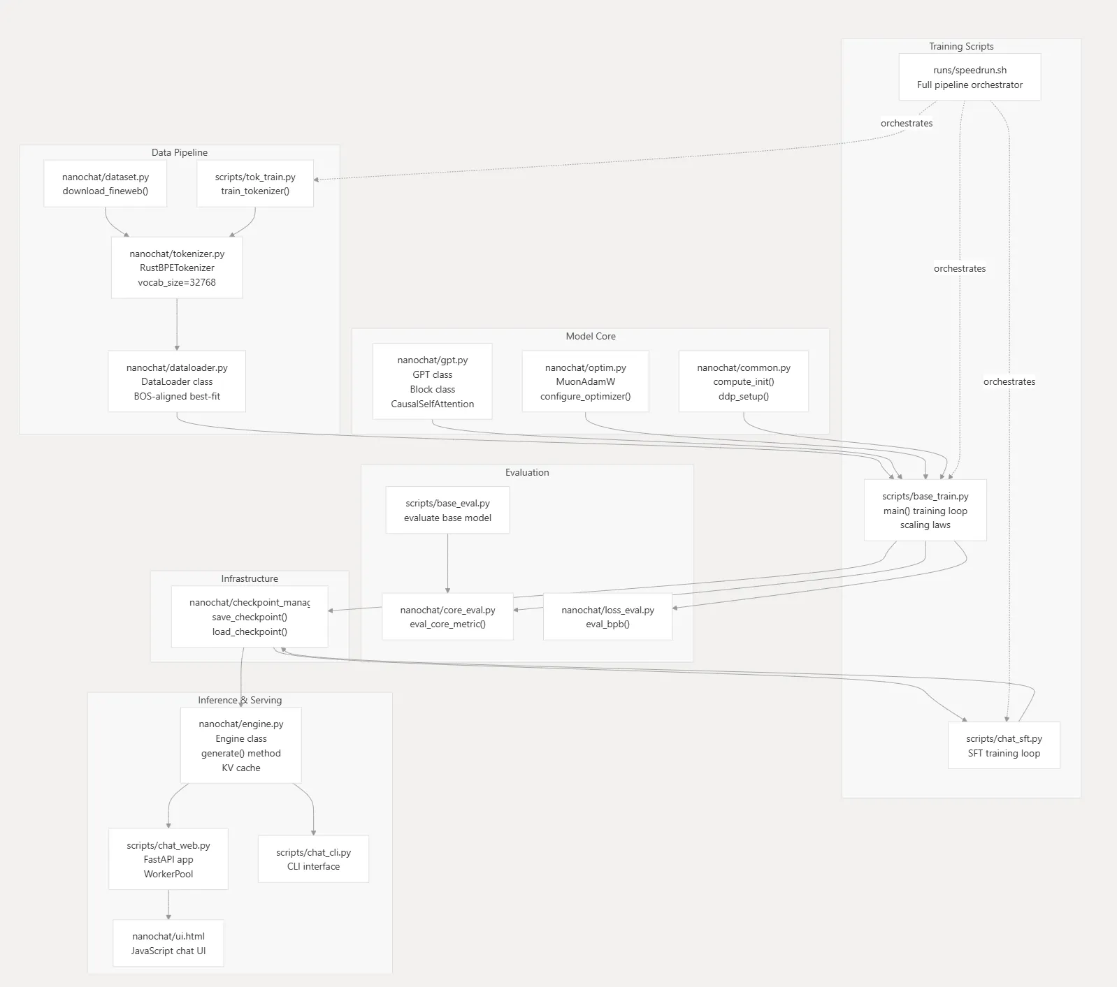
这是 Deepwiki 给 nanochat 画的架构图:run/speedrun.sh 脚本串起了 4 个模块。我们先从文件/类的级别来看一下这些模块:
-
数据处理(Data pipeline):
nanochat/dataset.py: 下载和管理 HuggingFace 数据集 (fineweb, smoltalk)scripts/tok_train.py:使用 tiktoken 库从 32K 词表训练一个 BPE Tokenizertokenizer.py: 封装训练好的 BPE Tokenizer,包含 special tokens(<|endoftext|>, <|user|>, <|assistant|>等)nanochat/dataloader.py: 数据打包:BOS对齐,best fit,实现 100% token 利用率
-
模型架构(Model Architecture):
nanochat/gpt.py: GPT 模型GPT: GPT Block 层,CausalSelfAttention:Flash Attention 3,SSSL,QK 归一化MLP:Feed-forward,ReLU² 激活函数- 其他架构特征…
nanochat/optim.py:优化器(MuonAdamW)
-
推理和服务(Inference and Serving):
nanochat/engine.py:KV-Cache 推理引擎scripts/chat-web.py: FastAPI 提供 web 服务,WorkerPool 支持并行推理nanochat/ui.html:前端页面
-
基础设施(Infrastructure):
nanochat/common.py: 分布式训练的初始化、清理、日志、设备检测等nanochat/checkpoint_manager.py管理模型检查点的S/Lnanochat/core_eval.py实现 CORE 评估指标计算
Speedrun
入手一个工程的第一步应该是将项目跑通。所以我问了AI,怎么跑通这个项目。我手里的计算资源是8张A800,每张卡80G显存。正好大过年的大家都没心思工作,这些卡就可以为我所用了。
帮我在 docs 里写一个文档,这个文档需要用中文详细讲解如何将这个项目跑通:1. speedrun.sh 都分为哪几步,做了哪些事情?2. 我在这个服务器上(`8*A800`)需要修改哪些配置等?这里得到的关键答案如下:
- A800 无法使用 FP8 精度,需要取消这个精度设置,使用默认的 BF16 精度。
- A800 好像不支持 Flash Attention 3,会自动回退到 SDPA (Scaled Dot Product Attention)(无需手动设置)。
可能因为这个原因,用默认参数实际训练了12小时,远超作者声称的3小时。
- 提前登录 wandb 以监控训练,并且记得使用 tmux/screen 运行长时命令。
这里贴出我修改后适配 A800 的 run/speedrun.sh 脚本:
#!/bin/bash
# This script is configured to train your own GPT-2 grade LLM (pretraining + finetuning)# It is designed to run on a blank 8XA800 GPU node and takes approximately 3 hours to complete.
# 1) Example launch (simplest):# bash runs/speedrun.sh# 2) Example launch in a screen session (because the run takes ~3 hours):# screen -L -Logfile runs/speedrun.log -S speedrun bash runs/speedrun.sh# 3) Example launch with wandb logging, but see below for setting up wandb first:# WANDB_RUN=speedrun screen -L -Logfile runs/speedrun.log -S speedrun bash runs/speedrun.sh
# Default intermediate artifacts directory is in ~/.cache/nanochatexport OMP_NUM_THREADS=1export NANOCHAT_BASE_DIR="$HOME/.cache/nanochat"mkdir -p $NANOCHAT_BASE_DIR
# -----------------------------------------------------------------------------# Python venv setup with uv
# install uv (if not already installed)command -v uv &> /dev/null || curl -LsSf https://astral.sh/uv/install.sh | sh# create a .venv local virtual environment (if it doesn't exist)[ -d ".venv" ] || uv venv# install the repo dependenciesuv sync --extra gpu# activate venv so that `python` uses the project's venv instead of system pythonsource .venv/bin/activate
# -----------------------------------------------------------------------------# wandb setup# If you wish to use wandb for logging (it's nice!, recommended).# 1) Make sure to first log in to wandb, e.g. run:# `wandb login`# 2) Set the WANDB_RUN environment variable when running this script, e.g.:# `WANDB_RUN=d26 bash speedrun.sh`if [ -z "$WANDB_RUN" ]; then # by default use "dummy" : it's handled as a special case, skips logging to wandb WANDB_RUN=dummyfi
# -----------------------------------------------------------------------------# During the course of the run, we will be writing markdown reports to the report/# directory in the base dir. This command clears it out and writes a header section# with a bunch of system info and a timestamp that marks the start of the run.python -m nanochat.report reset
# -----------------------------------------------------------------------------# Tokenizer
# Download the first ~2B characters of pretraining dataset# each data shard is ~250M chars# so we download 2e9 / 250e6 = 8 data shards at this point# each shard is ~100MB of text (compressed), so this is about ~800MB of data on disk# look at dev/repackage_data_reference.py for details on how this data was preparedpython -m nanochat.dataset -n 8# Immediately also kick off downloading more shards in the background while tokenizer trains# Approximately 350 shards are needed for 10B tokens of data for pretraining.# The maximum total number of shards available in the entire dataset is 1822.python -m nanochat.dataset -n 370 &DATASET_DOWNLOAD_PID=$!# train the tokenizer with vocab size 2**15 = 32768 on ~2B characters of datapython -m scripts.tok_train# evaluate the tokenizer (report compression ratio etc.)python -m scripts.tok_eval
# -----------------------------------------------------------------------------# Base model (pretraining)echo "Waiting for dataset download to complete..."wait $DATASET_DOWNLOAD_PID
# d24 model (slightly overtrained is enough to beat GPT-2 => increase data:params ratio from compute optimal 10.5 (default) to 12)# MODIFIED FOR A800: Removed --fp8 flagtorchrun --standalone --nproc_per_node=8 -m scripts.base_train -- --depth=26 --target-param-data-ratio=8.25 --device-batch-size=16 --run=$WANDB_RUN# evaluate the model: CORE metric, BPB on train/val, and draw samplestorchrun --standalone --nproc_per_node=8 -m scripts.base_eval -- --device-batch-size=16
# -----------------------------------------------------------------------------# SFT (teach the model conversation special tokens, tool use, multiple choice)
# download 2.3MB of synthetic identity conversations to impart a personality to nanochat# see dev/gen_synthetic_data.py for details on how this data was prepared and to get a sense of how you can easily tune itcurl -L -o $NANOCHAT_BASE_DIR/identity_conversations.jsonl https://karpathy-public.s3.us-west-2.amazonaws.com/identity_conversations.jsonl
# run SFT and eval the modeltorchrun --standalone --nproc_per_node=8 -m scripts.chat_sft -- --device-batch-size=16 --run=$WANDB_RUNtorchrun --standalone --nproc_per_node=8 -m scripts.chat_eval -- -i sft
# chat with the model over CLI! Leave out the -p to chat interactively# python -m scripts.chat_cli -p "Why is the sky blue?"
# even better, chat with your model over a pretty WebUI ChatGPT style# python -m scripts.chat_web
# -----------------------------------------------------------------------------# Generate the full report by putting together all the sections# report.md is the output and will be copied to current directory for conveniencepython -m nanochat.report generate总结一下这个速通脚本的流程:
- python 环境的初始化和依赖安装
- wandb 监控配置
- 下载第一个 ~2B 字符的预训练数据集
- 启动 tokenizer 的训练和评估,同时并行下载其余的预训练数据集(共370B)
- 预训练基础模型
- 评估基础模型
- 下载合成身份对话数据集
- 运行 SFT 训练
- 评估 SFT 模型
- 生成报告
Tokenizer
我们按照速通脚本的流程,从 tokenizer 开始。
nanochat 与 GPT-2 模型的 tokenizer 都使用了 BPE(Byte Pair Encoding) 算法训练。BPE 的“训练”过程其实并不是机器学习的训练,而是基于统计的确定性贪心算法,这有些类似 Huffman 编码:不断合并出现频数最高的一对字节,直到合并成目标的词表大小。
预分词
同时,nanochat 采用了类似 GPT-4 的预分词策略:
SPLIT_PATTERN = r"""'(?i:[sdmt]|ll|ve|re)|[^\r\n\p{L}\p{N}]?+\p{L}+|\p{N}{1,2}| ?[^\s\p{L}\p{N}]++[\r\n]*|\s*[\r\n]|\s+(?!\S)|\s+"""(?i:[sdmt]|ll|ve|re): 匹配’s, ‘d, ‘m, ‘t, ‘ll, ‘ve, ‘re 等常见英语后缀[^\r\n\p{L}\p{N}]?+\p{L}+: 匹配单词,允许单词前有一个非换行、非字母数字的字符\p{N}{1,2}: 匹配 1 到 2 个数字, 这时一个关键优化,避免语料库中的无意义长数字污染token- …
基于字节对的BPE可以解决 OOV(Out-Of-Vocabulary) 问题:总能把未知词拆成已知字节;预分词一定程度上缓解了形态学缺失问题:如果合并完全基于统计,有时会拆出没有意义的片段(如 the 拆成 t + he)。
RustBPE
实现细节可以看 RustBPE。 这里简单介绍一下 RustBPE 实现上的优化:
1. 预处理
预处理包含了预分词与统计预分词之后得到的词块的词频。这里有两个系统问题需要解决:
- 内存:直接将整个语料加载到内存会撑爆内存,因此进行分块缓冲处理。这一步不断拉取
buffer_size个字符串,持有 GIL,是单线程。 - 时间:这里对加载到内存缓冲区的每一组语料使用 Rust 的并发模型 (Rayon, map-reduce) 来实现并行预分词(正则切分)和局部词频汇总。释放 GIL 之后,在 map 阶段,每个线程拥有私有的词频统计哈希表,可以并行地进行正则切分和局部词频统计;在 reduce 阶段,也会树状合并以上产生的局部词频计数表。
主循环部分的代码摘录如下:
// Stream ingestion loop: refill under GIL, process without GIL (parallel) loop { let exhausted = refill(&mut buf)?; if buf.is_empty() && exhausted { break; }
total_sequences += buf.len() as u64;
let pattern = self.compiled_pattern.clone(); let local: AHashMap<CompactString, i32> = py.detach(|| { buf.par_iter() .map(|s| { let mut m: AHashMap<CompactString, i32> = AHashMap::new(); for mat in pattern.find_iter(s) { let piece = mat.expect("regex match failed").as_str(); *m.entry(CompactString::from(piece)).or_default() += 1; } m }) .reduce(AHashMap::new, |mut a, b| { for (k, v) in b { *a.entry(k).or_default() += v; } a }) });
// Merge local into global (single-threaded) for (k, v) in local { *counts.entry(k).or_default() += v; }
if exhausted { break; } }2. 核心训练
这一步实现了基于优先队列的增量更新算法,即每次合并出现频数最高的一对字节对。输入包含了预处理阶段得到的词块words和它们的词频counts。
建堆
接下来BPE的算法会在预分词的产物词块上进行合并。每一个词块 Word 存储了这个词块的字节序列,通过 Vec<u32> 的有序排列保留了字节级别的“谁在谁旁边”的信息。建堆之前,调用 count_pairs_parallel ,通过 map-reduce 的方式统计出全局的两张地图:
pair_counts: Pair → 总频数where_to_update: Pair → 词块位置(在words中的索引)
堆中的元素被封装成任务包, 每个任务包包含了一个待合并的 Pair、这个 Pair 的频数以及这个Pair 关联到的所有词块位置。
struct MergeJob { pair: Pair, count: u64, /// set of word indices where this pair may occur and needs processing pos: AHashSet<usize>,}Karpathy 这里采用了 Octonary Heap, 大规模数据排序相比二叉堆堆的高度更矮,可以减少CPU Cache Miss。
合并
核心流程控制:Lazy Refresh(懒更新)。这里依赖了全局的 pair_counts, 这个哈希表记录了当前时刻最准确、最新的 Pair 频数。
- 在每个 MergeJob 执行合并时,立即通过
top.pos的信息追溯并进行全量的副作用传播。 - 在每个 MergeJob 执行合并前,先检查堆顶的 counts 是否与全局的真实
pair_counts一致,如果不一致,需要更新成最新的频数,然后重新压入队列。
impl Tokenizer { /// Core incremental BPE training given unique words and their counts. /// `words`: one entry per unique chunk (Vec<u32> of token-ids/bytes). /// `counts`: same length as `words`, count per chunk. fn train_core_incremental(&mut self, mut words: Vec<Word>, counts: Vec<i32>, vocab_size: u32) { assert!(vocab_size >= 256, "vocab_size must be at least 256"); let num_merges = vocab_size - 256; log::info!("Starting BPE training: {} merges to compute", num_merges); self.merges.clear();
// ---- Initial pair_counts and where_to_update (parallel) ---- log::info!( "Computing initial pair counts from {} unique sequences", words.len() ); let (mut pair_counts, mut where_to_update) = count_pairs_parallel(&words, &counts);
// ---- Build heap ---- log::info!("Building heap with {} unique pairs", pair_counts.len()); let mut heap = OctonaryHeap::with_capacity(pair_counts.len()); for (pair, pos) in where_to_update.drain() { let c = *pair_counts.get(&pair).unwrap_or(&0); if c > 0 { heap.push(MergeJob { pair, count: c as u64, pos, }); } }
// ---- Merge loop ---- log::info!("Starting merge loop"); let mut merges_done = 0u32; let mut last_log_percent = 0u32;
while merges_done < num_merges { let Some(mut top) = heap.pop() else { break; };
// Lazy refresh: if the count changed since we queued this job, update and requeue let current = *pair_counts.get(&top.pair).unwrap_or(&0); if current <= 0 { // Pair no longer exists or has non-positive count, skip it continue; } if top.count != current as u64 { top.count = current as u64; heap.push(top); continue; }
// Record merge let new_id = 256 + merges_done; self.merges.insert(top.pair, new_id);
// Merge this pair in all words where it occurs let mut local_pos_updates: AHashMap<Pair, AHashSet<usize>> = AHashMap::new(); for &word_idx in &top.pos { // Apply merge to this word and collect pair-count deltas let changes = words[word_idx].merge_pair(top.pair, new_id); // Update global pair counts based on this word's count for (pair, delta) in changes { let delta_total = delta * counts[word_idx]; if delta_total != 0 { *pair_counts.entry(pair).or_default() += delta_total; if delta > 0 { local_pos_updates.entry(pair).or_default().insert(word_idx); } } } }
// Add the updated pair counts back to the heap for (pair, pos) in local_pos_updates { let cnt = *pair_counts.get(&pair).unwrap_or(&0); if cnt > 0 { heap.push(MergeJob { pair, count: cnt as u64, pos, }); } }
merges_done += 1;
// Log progress every 1% let current_percent = (merges_done * 100) / num_merges; if current_percent > last_log_percent { log::info!( "Progress: {}% ({}/{} merges) - Last merge: {:?} -> {} (frequency: {})", current_percent, merges_done, num_merges, top.pair, new_id, top.count ); last_log_percent = current_percent; } }
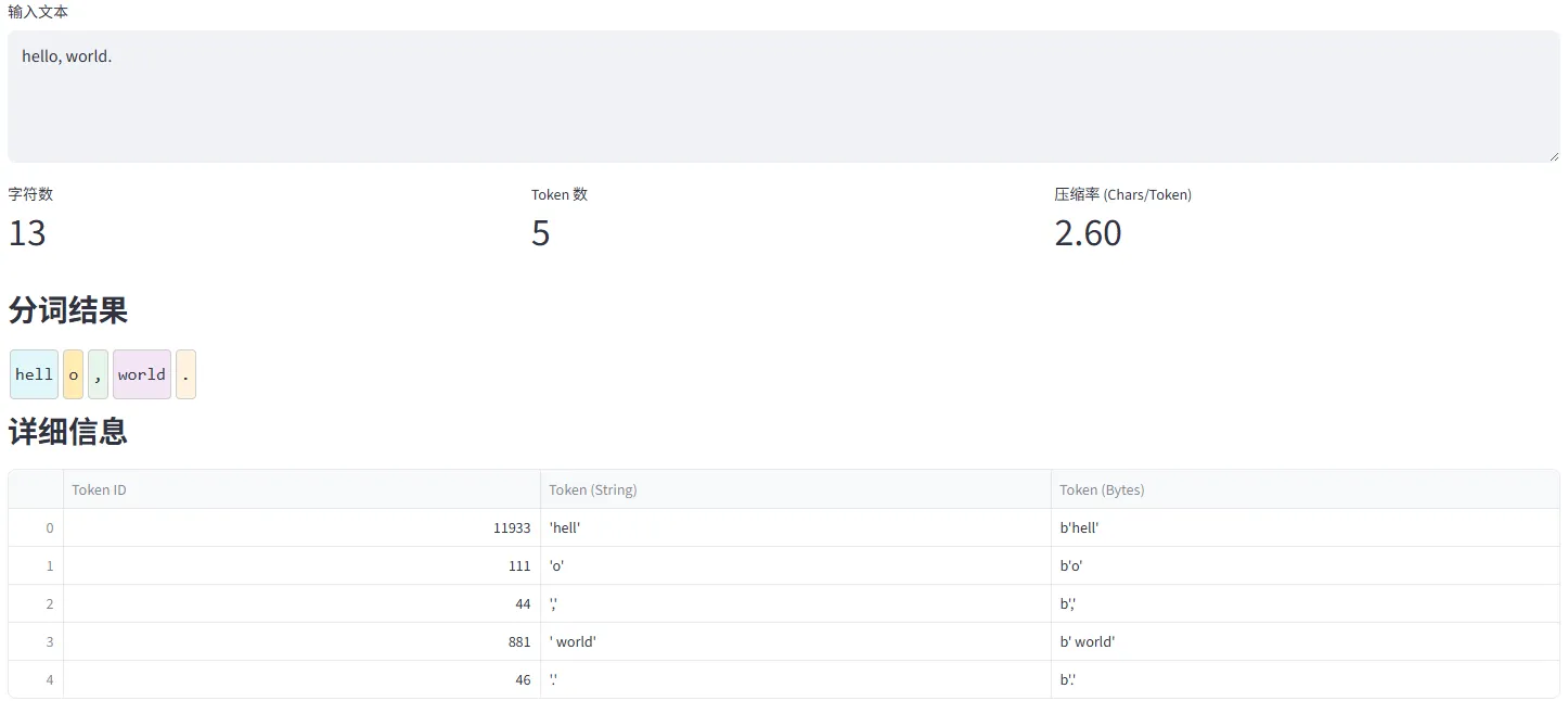
log::info!("Finished training: {} merges completed", merges_done); }}训练完成后,就可以通过 tiktoken 引擎对照训练产出的词表和分词规则表,将输入的文本转为token. 一个简单例子可视化如下图:
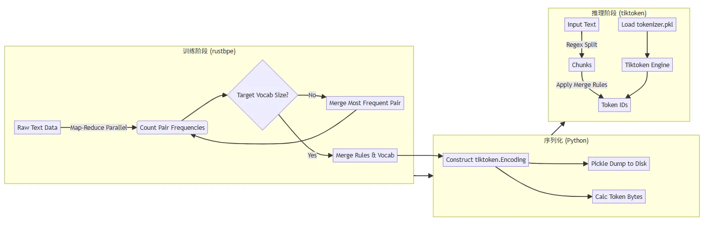
最后一张图总结 nanochat tokenizer 的训练和推理流程:
Model
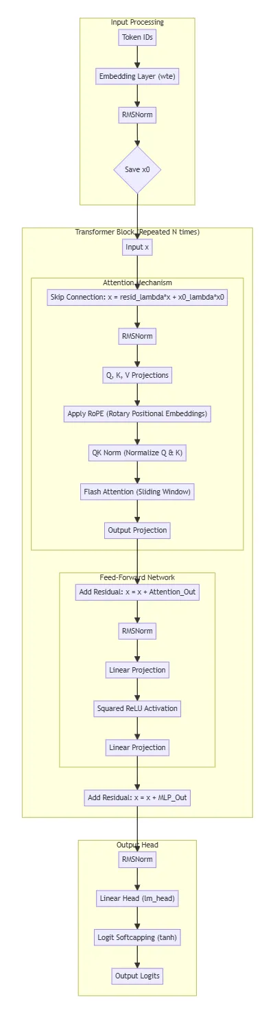
模型架构如下图:
我们可以从class GPT的前向传播入手:
def forward(self, idx, targets=None, kv_cache=None, loss_reduction='mean'): B, T = idx.size()
# Grab the rotary embeddings for the current sequence length (they are of shape (1, seq_len, 1, head_dim/2)) assert T <= self.cos.size(1), f"Sequence length grew beyond the rotary embeddings cache: {T} > {self.cos.size(1)}" assert idx.device == self.cos.device, f"Rotary embeddings and idx are on different devices: {idx.device} != {self.cos.device}" assert self.cos.dtype == torch.bfloat16, "Rotary embeddings must be in bfloat16" # if kv cache exists, we need to offset the rotary embeddings to the current position in the cache T0 = 0 if kv_cache is None else kv_cache.get_pos() cos_sin = self.cos[:, T0:T0+T], self.sin[:, T0:T0+T] # truncate cache to current sequence length
# Forward the trunk of the Transformer x = self.transformer.wte(idx) # embed current token x = norm(x) x0 = x # save initial normalized embedding for x0 residual for i, block in enumerate(self.transformer.h): x = self.resid_lambdas[i] * x + self.x0_lambdas[i] * x0 ve = self.value_embeds[str(i)](idx) if str(i) in self.value_embeds else None x = block(x, ve, cos_sin, self.window_sizes[i], kv_cache) x = norm(x)
# Forward the lm_head (compute logits) softcap = 15 # smoothly cap the logits to the range [-softcap, softcap] logits = self.lm_head(x) # (B, T, padded_vocab_size) <- very big tensor, large amount of memory logits = logits[..., :self.config.vocab_size] # slice to remove padding logits = logits.float() # switch to fp32 for logit softcap and loss computation logits = softcap * torch.tanh(logits / softcap) # squash the logits
if targets is not None: # training: given the targets, compute and return the loss # TODO experiment with chunked cross-entropy? loss = F.cross_entropy(logits.view(-1, logits.size(-1)), targets.view(-1), ignore_index=-1, reduction=loss_reduction) return loss else: # inference: just return the logits directly return logits以上的GPT前向传播过程可以分为 3 部分:
- Input Processing: 对输入进行预处理,包括 token embedding 和归一化。
- Transformer Blocks: 包含多个 Transformer Block,每个 Block 包含 Attention Mechanism 和 Feed-Forward Network。
- Output Processing: 对 Transformer 的输出进行处理,包括归一化和 lm_head 计算 logits。
Input Processing
这里做的处理有三步:
- Weight Token Embedding: 将输入的 token 序列转化为
n_embd维的向量。这里的 WTE 是一个表格,即Shape(padded_vocab_size, n_embd)的矩阵,每个 token 对应了一个n_embd维的向量。为什么要做这个 Embedding?
- token是一个离散的数,难以表达 token 的复杂语义信息。因此需要映射到一个高维向量,使得模型通过学习 WTE 的权重就可以表达 token 的语义信息。
- norm(x): 对输入进行初始归一化。 使用 RMSNorm,即对每个词向量的维度进行归一化,公式为: 注:LayerNorm 与 RMSNorm 的区别在于,前者会进行偏移(中心化)和缩放,而后者只根据 RMS 来缩放。因此后者无需计算均值和方差,大大减少了计算量,两者效果也一般无明显差异。 其中, 和 是可学习的参数,用于缩放(和偏移)归一化后的向量。nanochat 在这一步的 RMSNorm 没有传入可学习的权重。
- Save x0: 保存归一化后的初始输入。
Transformer Blocks(核心)
这部分是模型的核心,包含了 Attention Mechanism 和 Feed-Forward Network 两个主要部分。
class Block(nn.Module): def __init__(self, config, layer_idx): super().__init__() self.attn = CausalSelfAttention(config, layer_idx) self.mlp = MLP(config)
def forward(self, x, ve, cos_sin, window_size, kv_cache): x = x + self.attn(norm(x), ve, cos_sin, window_size, kv_cache) x = x + self.mlp(norm(x)) return xAttention Mechanism
关于 Attention 机制,Lil’s Log这篇讲得很好。直观地理解,这种机制可以通过重要性权重表达元素之间的相关性。而 self-attention 则表示了序列中每个元素与其他所有元素之间的交互关系和依赖强度。
In a nutshell, attention in deep learning can be broadly interpreted as a vector of importance weights: in order to predict or infer one element, such as a pixel in an image or a word in a sentence, we estimate using the attention vector how strongly it is correlated with (or “attends to” as you may have read in many papers) other elements and take the sum of their values weighted by the attention vector as the approximation of the target.
以下是 nanochat 的 attention 模块源码
class CausalSelfAttention(nn.Module): def __init__(self, config, layer_idx): super().__init__() self.layer_idx = layer_idx self.n_head = config.n_head self.n_kv_head = config.n_kv_head self.n_embd = config.n_embd self.head_dim = self.n_embd // self.n_head assert self.n_embd % self.n_head == 0 assert self.n_kv_head <= self.n_head and self.n_head % self.n_kv_head == 0 self.c_q = nn.Linear(self.n_embd, self.n_head * self.head_dim, bias=False) self.c_k = nn.Linear(self.n_embd, self.n_kv_head * self.head_dim, bias=False) self.c_v = nn.Linear(self.n_embd, self.n_kv_head * self.head_dim, bias=False) self.c_proj = nn.Linear(self.n_embd, self.n_embd, bias=False) self.ve_gate_channels = 32 self.ve_gate = nn.Linear(self.ve_gate_channels, self.n_kv_head, bias=False) if has_ve(layer_idx, config.n_layer) else None
def forward(self, x, ve, cos_sin, window_size, kv_cache): B, T, C = x.size()
# Project the input to get queries, keys, and values # Shape: (B, T, H, D) - FA3's native layout, no transpose needed! q = self.c_q(x).view(B, T, self.n_head, self.head_dim) k = self.c_k(x).view(B, T, self.n_kv_head, self.head_dim) v = self.c_v(x).view(B, T, self.n_kv_head, self.head_dim)
# Value residual (ResFormer): mix in value embedding with input-dependent gate per head if ve is not None: ve = ve.view(B, T, self.n_kv_head, self.head_dim) gate = 2 * torch.sigmoid(self.ve_gate(x[..., :self.ve_gate_channels])) # (B, T, n_kv_head), range (0, 2) v = v + gate.unsqueeze(-1) * ve
# Apply Rotary Embeddings to queries and keys to get relative positional encoding cos, sin = cos_sin q, k = apply_rotary_emb(q, cos, sin), apply_rotary_emb(k, cos, sin) q, k = norm(q), norm(k) # QK norm
# Flash Attention (FA3 on Hopper+, PyTorch SDPA fallback elsewhere) # window_size is (left, right) tuple: (N, 0) for causal, (-1, 0) for full context if kv_cache is None: # Training: causal attention with optional sliding window y = flash_attn.flash_attn_func(q, k, v, causal=True, window_size=window_size) else: # Inference: use flash_attn_with_kvcache which handles cache management k_cache, v_cache = kv_cache.get_layer_cache(self.layer_idx) y = flash_attn.flash_attn_with_kvcache( q, k_cache, v_cache, k=k, v=v, cache_seqlens=kv_cache.cache_seqlens, causal=True, window_size=window_size, ) # Advance position after last layer processes if self.layer_idx == kv_cache.n_layers - 1: kv_cache.advance(T)
# Re-assemble the heads and project back to residual stream y = y.contiguous().view(B, T, -1) y = self.c_proj(y) return ySelf-Attention
首先回顾注意力的计算公式:通过训练模型,我们学习到了查询矩阵 、键矩阵 和值矩阵 。这三个矩阵的维度分别为 、 和 。其中 是模型的隐藏维度(也就是词向量的维度), 是查询向量或键向量的维度, 是值向量的维度。
计算注意力分数的点积形式 就要求了 ,一般也会让 。
另外,在计算注意力分数时,我们通常会对其进行归一化,以确保 softmax 函数的输入在合理的范围内,避免过大的分数导致 softmax 梯度。这通常是通过对分数进行缩放来实现的,即 。
-
Softmax 函数将输入向量 映射为概率分布 。对于其中第 个元素的计算公式为:
当我们求 Softmax 的梯度时,公式如下:, 也就是:
- 当 时:
- 当 时:
-
因此,分母上的 就是为了保证高维空间中点积的结果不会过大,以防止 softmax 之后的分布接近 one-hot,导致反向传播的梯度消失。
Grouped Query Attention
从MHA到GQA的科普,可以参考苏剑林对 DeepSeek 所作创新 MLA 介绍的博客文章:缓存与效果的极限拉扯:从MHA、MQA、GQA到MLA
在讨论之前我们先在代码中明确:
B, T, C = x.size()Attention 层的输入 x 的形状为(B:Batch size、T:Token 序列长度、C:词向量维度,即 n_embd 即 )。
相比单头注意力,MHA 并不是对计算效率的优化,而是出于模型表达能力的考虑。每个 Head 是一个独立的小空间,都有自己的、、,最终也是独立地计算 softmax,因此可以在序列中并行计算捕捉不同位置的信息。从直觉来看,这样可以有效地缓解 softmax 极其排他、容易形成 one-hot 的数学特性。
MHA 的本质是并行运行 个 attention 单元,并将结果缝合:
其中每一个头 都是独立投影的结果:
随着 Token 序列长度的增加,MHA 会面临显存问题:对每个 Head 都需要存储一套 形状为 的矩阵。(, 即 即 n_embed),因此带来了 KV cache 存储的大量显存需求。MQA 和 GQA 就是为了在显存上优化这个问题:
- GQA:将众多的 Query 头进行分组(Group)。每一组 Query 头共享一对特定的 头。
- MQA:将显存优化到极限,也就是 GQA 中 的情况,但是这样模型会变笨。
表格对比如下:
| 机制 | Query 头数 | KV 头数 | 显存压力 | 表达能力 | 代表模型 |
|---|---|---|---|---|---|
| MHA | 极大 | 极强 | GPT-3, Transformer 原型 | ||
| MQA | 极低 | 较弱 | PaLM, Falcon (部分) | ||
| GQA | () | 低 | 强 (接近 MHA) | Llama 3, NanoChat |
我们结合代码看一下 nanochat 中 GQA 的具体实现:(见注释)
初始化:
class CausalSelfAttention(nn.Module): def __init__(self, config, layer_idx): super().__init__() self.layer_idx = layer_idx self.n_head = config.n_head # Query 的头数 (h) self.n_kv_head = config.n_kv_head # Key/Value 的头数 (g) self.n_embd = config.n_embd # 嵌入维度 (C 或 d_model)
# 每个头的维度:C = n_head * head_dim,确保多头拼接后能还原回 C self.head_dim = self.n_embd // self.n_head
# 健壮性检查:确保嵌入维度能被头数整除 assert self.n_embd % self.n_head == 0
# GQA 核心约束:KV 头数必须小于等于 Q 头数,且能被整除(实现均匀分组) # 如果 n_kv_head = 1,则是 MQA;如果 n_kv_head = n_head,则是 MHA assert self.n_kv_head <= self.n_head and self.n_head % self.n_kv_head == 0
# Q 投影层:输出维度为 n_head * head_dim,即保持完整的 C self.c_q = nn.Linear(self.n_embd, self.n_head * self.head_dim, bias=False)
# K/V 投影层(GQA 的精髓):输出维度大大缩小,仅为 n_kv_head * head_dim # 这里的输出宽度直接决定了 KV Cache 的显存占用量 self.c_k = nn.Linear(self.n_embd, self.n_kv_head * self.head_dim, bias=False) self.c_v = nn.Linear(self.n_embd, self.n_kv_head * self.head_dim, bias=False)
# 输出投影层 (Wo):负责将所有头拼接后的结果融合,重新映射回 n_embd 空间 self.c_proj = nn.Linear(self.n_embd, self.n_embd, bias=False)# ...前向传播
def forward(self, x, ve, cos_sin, window_size, kv_cache): B, T, C = x.size()
# Project the input to get queries, keys, and values # Shape: (B, T, H, D) - FA3's native layout, no transpose needed!
# q 被拆成 n_head 个头,每个头的维度是 head_dim # k,v 被分成 g 组,每个组有 n_kv_head 个头,每个头的维度是 head_dim, g = n_head // n_kv_head q = self.c_q(x).view(B, T, self.n_head, self.head_dim) k = self.c_k(x).view(B, T, self.n_kv_head, self.head_dim) v = self.c_v(x).view(B, T, self.n_kv_head, self.head_dim)
# Value residual (ResFormer): mix in value embedding with input-dependent gate per head # ...
# Apply Rotary Embeddings to queries and keys to get relative positional encoding # ...
# Flash Attention (FA3 on Hopper+, PyTorch SDPA fallback elsewhere) # 训练 / 推理 分别调用 flash-attention 算子,其中推理有 kv cache
# Re-assemble the heads and project back to residual stream
# 将输出 y 的形状重新转换为 (B, T, C) y = y.contiguous().view(B, T, -1)
# c_proj 是一个全连接层,它让来自不同头的特征进行第一次实质性的加权混合 # 同时还将注意力层的输出通过线性变换,调整到适合与原始输入 $x$ 进行**残差相加(Residual Add)**的状态 y = self.c_proj(y) return y这里也给出GQA的形式化表达方便理解:假设我们有 个 Query 头,但只有 个 KV 头(其中 且 能被 整除):
关键在于每个头 的计算方式:
其中:
- :这是一个索引映射函数。它表示第 个 Query 头对应的是第 组 KV 头。
与代码中的变量对应如下:
- :
self.n_head(Query 总头数) - :
self.n_kv_head(KV 总头数) - : 每个组的大小 (Group Size)。一个 Query 头对应 个 KV 头。
- : 对应
self.c_q中第 个头的权重。 - : 对应
self.c_k中属于该组的那一小块权重。 - : 对应
self.c_v中属于该组的那一小块权重。 - :对应代码里的
y.view(B, T, -1)。 - :对应代码里的
self.c_proj
Causual Attention
主流的自回归 LLM 使用 Causual Attention, 也就是做 next-token-prediction 时,只关注当前位置和之前的 tokens,而不关注之后的 tokens。
其中, 是一个上三角矩阵, 当 ,否则 。在计算注意力分数时, 被加到 上,使得对应的 softmax 值为 。
FlashAttention V3 算子和 pytorch 的 SDPA torch.nn.functional.scaled_dot_product_attention 函数,都直接支持 Causual Attention。
# flash_attn_func ...return _fa3.flash_attn_func(q, k, v, causal=causal, window_size=window_size)
# sdpa_attention ...return F.scaled_dot_product_attention(q, k, v, attn_mask=mask, enable_gqa=enable_gqa)(FA3 内核会自动识别这是 Grouped-Query Attention (GQA) 模式,并自动执行广播(Broadcasting)逻辑,将每个 KV Head 对应到多个 Q Head 上,因此没有显式地传入 enable_gqa 参数)
RoPE
RoPE (Rotary Positional Embedding,旋转位置编码) 是目前最主流的位置编码技术。
在 Transformer 中,Attention 机制本身是位置无关的(词序打乱结果一样)。为了让模型理解顺序,我们需要加入位置信息:
- 绝对位置编码 (Absolute PE): 给每个位置加一个固定的向量(如 BERT、GPT-2)。缺点是无法很好地处理超出训练长度的文本。
- 相对位置编码 (Relative PE): 关注词之间的距离。虽然效果好,但在计算时往往效率较低,且难以与旋转计算这种数学上的优雅特性结合。
想象二维空间中的两个向量 和 。RoPE 会根据它们所在的位置 和 ,分别对它们进行旋转。如果我们将 旋转 角度,将 旋转 角度。它们之间的夹角就变成了 。由于 Attention 的核心是计算 和 的内积(点积),而内积的大小取决于它们之间的夹角。因此,计算结果只与它们的相对距离 有关。
注入位置信息后的 向量内积为:
注意: 在高维空间中,RoPE 将维度两两分组,每一组都在各自的复平面上进行这种“旋转”操作。
苏剑林的博客也给出了一种直观的理解方式:RoPE是一种β进制编码
在 nanochat 中,RoPE的实现如下:
- 预处理阶段,预先处理出
(1, T, 1, D//2)形状的 cos 和 sin 向量, - 计算 , 的位置编码时,将输入序列 x
(B, T, H, D)拆分成两组 x1, x2(B, T, H, D//2), 然后对 x1 和 x2 分别配对施加二维旋转矩阵 (只有二维,相当于复数乘法可以手动拆开计算)。
def apply_rotary_emb(x, cos, sin): assert x.ndim == 4 # multihead attention d = x.shape[3] // 2 x1, x2 = x[..., :d], x[..., d:] # split up last dim into two halves y1 = x1 * cos + x2 * sin # rotate pairs of dims (正负号这里不重要,看起来是实现的顺时针旋转) y2 = x1 * (-sin) + x2 * cos return torch.cat([y1, y2], 3)
# ...
def _precompute_rotary_embeddings(self, seq_len, head_dim, base=10000, device=None): # TODO: bump base theta more? e.g. 100K is more common more recently # autodetect the device from model embeddings if device is None: device = self.transformer.wte.weight.device # stride the channels channel_range = torch.arange(0, head_dim, 2, dtype=torch.float32, device=device) inv_freq = 1.0 / (base ** (channel_range / head_dim)) # stride the time steps t = torch.arange(seq_len, dtype=torch.float32, device=device) # calculate the rotation frequencies at each (time, channel) pair freqs = torch.outer(t, inv_freq) cos, sin = freqs.cos(), freqs.sin() cos, sin = cos.bfloat16(), sin.bfloat16() # keep them in bfloat16 cos, sin = cos[None, :, None, :], sin[None, :, None, :] # add batch and head dims for later broadcasting return cos, sinValue Residual
传统的 Transformer 结构中,残差连接(Residual Connection)通常包裹在整个 Attention 块的外面:
而 ResFormer (Value Residual) 认为这还不够。它在 Attention 内部的 (Value)计算中又加了一层残差,使得同时能表达上下文信息和原始输入的含义。
def has_ve(layer_idx, n_layer): """Returns True if GPT layer should have Value Embedding (alternating, last layer always included).""" return layer_idx % 2 == (n_layer - 1) % 2
# ...
self.ve_gate_channels = 32 self.ve_gate = nn.Linear(self.ve_gate_channels, self.n_kv_head, bias=False) if has_ve(layer_idx, config.n_layer) else None
# ...
# Value residual (ResFormer): mix in value embedding with input-dependent gate per head if ve is not None: ve = ve.view(B, T, self.n_kv_head, self.head_dim) gate = 2 * torch.sigmoid(self.ve_gate(x[..., :self.ve_gate_channels])) # (B, T, n_kv_head), range (0, 2) v = v + gate.unsqueeze(-1) * ve在 nanochat 中,transformer blocks 的最后一层一定有 Value Residual, 向前隔一层才会做一次 Value Residual. 以上代码实现了 Value Residual,即将原始输入 经过门控网络调节后,与投影后的 相加。
对于第 个位置的第 个注意力头:
-
:输入向量 在时间步 的前 32 个特征通道。
-
:门控矩阵,它只与这 32 个维度发生作用。
Feed-Forward Network
class MLP(nn.Module): def __init__(self, config): super().__init__() self.c_fc = nn.Linear(config.n_embd, 4 * config.n_embd, bias=False) self.c_proj = nn.Linear(4 * config.n_embd, config.n_embd, bias=False)
def forward(self, x): x = self.c_fc(x) x = F.relu(x).square() x = self.c_proj(x) return xFFN 层的实现非常简单:它是一个 MLP :2个全连接层中间经过有一层激活函数,也就是一个升维 - 激活 - 降维的过程。
Output Processing
经过多轮的 Transformer Blocks 的前向传播之后,就来到了最终的输出层。截取 GPT 类的 forward 方法中最后处理输出的部分如下:
x = norm(x)
# Forward the lm_head (compute logits) softcap = 15 # smoothly cap the logits to the range [-softcap, softcap] logits = self.lm_head(x) # (B, T, padded_vocab_size) <- very big tensor, large amount of memory logits = logits[..., :self.config.vocab_size] # slice to remove padding logits = logits.float() # switch to fp32 for logit softcap and loss computation logits = softcap * torch.tanh(logits / softcap) # squash the logits
if targets is not None: # training: given the targets, compute and return the loss # TODO experiment with chunked cross-entropy? loss = F.cross_entropy(logits.view(-1, logits.size(-1)), targets.view(-1), ignore_index=-1, reduction=loss_reduction) return loss else: # inference: just return the logits directly return logits-
LM Head 线性投影
首先,通过
lm_head这个全连接层,将经过归一化(Norm)的隐藏状态向量 投影到词表空间:-
:位置 的特征向量。
-
:输出层权重矩阵( 是对齐后的词表大小)。
-
:原始 Logits 向量。
-
-
词表切片
由于为了计算效率进行了填充(Padding),我们需要将向量截断回实际词表大小 :
-
Logits 软截断(Logit Softcapping)
这是代码中最关键的非线性变换,旨在将 Logits 限制在区间 内(代码中 ):
- 当原始 Logit 非常大时,,结果趋近于 ;当其非常小时,结果趋近于 。这防止了模型产生极其极端的概率分布。
-
模型输出用于训练/推理
- 训练时,通过 logits 计算交叉熵损失(
F.cross_entropy) - 推理时,直接返回 logits 向量,用于下游的采样,以生成下一个 token。
- 训练时,通过 logits 计算交叉熵损失(
至此,我们走完了模型的整个前向传播过程,也就理解了 nanochat 的模型架构。
Data & Pretraining
在这部分,我们主要关注以下三个内容:
- 大模型如何进行预训练?
- 训练过程使用的优化器
- 大模型在预训练上的工程优化
预训练
大模型的自监督预训练(Self-Supervised Pre-training)的核心任务是 Next Token Prediction(下一个词预测) ,即通常所说的 Causal Language Modeling (CLM) 。模型根据当前的上下文 预测下一个 token 。
错位切分
自监督意味着不需要人工标注标签, 数据本身就是标签 。 我们将一段文本序列错位切分:
为了将这段描述转化为专业的数学形式,通常我们使用序列符号 来表示文本中的 Token。以下是优化后的数学定义:
假设给定一个长度为 的 Token 序列 ,在自监督预训练(因果语言模型)中,输入与目标的关系定义如下:
-
输入序列 (Input, ):
即序列的前 个 Token。
-
目标序列 (Target, ):
即序列向后平移一位后的 个 Token。
-
训练任务: 对于每一个时间步 ,模型根据当前及之前的输入预测下一个 Token:
此时,正确答案(Ground Truth) 即为目标序列中对应位置的值:
在计算损失函数(如交叉熵损失)时,模型实际上是在优化以下目标:
数据打包
在预训练阶段,nanochat 使用 BOS-aligned Best-Fit 算法,
- 从缓冲区中,选择能放入剩余空间且长度最大的文档(最佳适配)
- 重复步骤1,直到没有文档能完整放入
- 当没有文档能完整放入时,选择最短的文档进行裁剪,恰好填满剩余空间
- 每行以 BOS token 开头
这样做有如下的特点:
- 100% 利用率 :无填充(padding),每个 token 都会被训练
- 约 35% token 被裁剪丢弃 :这是为了保证每行都以 BOS 开头
- 每行都能看到完整上下文 :因为都从 BOS 开始
DDP(Distributed Data Parallel)
1. 单卡训练 (baseline)
在只有一张GPU的时候,训练模型非常简单:
- 数据:Dataloader 按顺序读取一小批数据 (例如 8 句话)
- 前向传播 (forward):将这 8 句话扔进模型,算出一个loss
- 反向传播 (backward):根据 loss 计算梯度
- 参数更新 (optimizer step):优化器 (如 AdamW) 根据梯度更模型参数
- 循环以上步骤,读取下一批数据…
2. 朴素的数据并行 (Data Parallel, DP)
现在有了 4 张 GPU,我们希望将训练速度提升 4 倍,最直观的想法就是数据并行(DP)。
- 模型复制:在4张卡上,各放一个相同的模型副本
- 数据分发:之前一次读8句话,现在可以一次读32句话,GPU0拿0-7,GPU1拿8-15,…
- 独立计算:4 张卡同时各自做前向传播和反向传播,各自计算出自己的梯度。
- 汇总更新:问题来了,如果4个GPU各自更新自己的模型,4个模型就长得不一样了!
此处的解决方法是:在更新梯度之前,让 4 张卡互相通信,求梯度的平均。(all reduce)
对应nanochat中的代码:
多卡无锁数据分发 每次从当前 rank 跳过 ddp_world_size
关于 rank
在分布式计算和深度学习(如 PyTorch DDP 或 MPI)中, Rank 指的是 进程的唯一标识符(ID) 。
在分布式训练时,我们会同时启动多个一模一样的程序副本(进程),通常一个进程对应控制一块 GPU。系统会为每个进程分配一个唯一的编号,这个编号就是 Rank 。
通常我们会接触到三个相关环境变量(这也是 torchrun 启动分布式训练时自动注入的):
Global Rank(全局 Rank,简称 Rank)
- 定义 :在所有参与训练的机器、所有 GPU 中的 全局唯一编号 。
- 范围 : 0 到 World Size - 1 。
- 作用 :用于全局协调。特别是 Rank 0 通常被称为主进程(Master Node),它会被赋予一些特权任务,比如:打印训练进度日志、下载数据集、保存模型权重(Checkpoint)等,以避免所有进程重复做这些写磁盘/打印的操作。
Local Rank(本地 Rank)
- 定义 :在当前物理机器(Node)内部的编号。
- 范围 : 0 到 该机器上的 GPU 数量 - 1 。
- 作用 :决定当前进程具体使用机器上的哪一块物理显卡。通常代码里会写 torch.cuda.set_device(local_rank) 。
World Size(世界大小/总进程数)
- 定义 :参与训练的总进程数量(通常等于总 GPU 数量)。
while True:# ... rg_idx = ddp_rank while rg_idx < pf.num_row_groups: rg = pf.read_row_group(rg_idx) batch = rg.column('text').to_pylist() for i in range(0, len(batch),tokenizer_batch_size): yield batch[i:i+tokenizer_batch_size],(pq_idx, rg_idx, epoch) rg_idx += ddp_world_size pq_idx += 1 first_pass = False epoch += 1梯度汇总(朴素做法)
对于模型中的小参数(如偏置项),nanochat直接采用最朴素的 all reduce:在 optim.py 中:
# ... grad = p.grad if p.numel() < 1024: # Small params: all_reduce (no scattergather needed) future = dist.all_reduce(grad, op=distReduceOp.AVG, async_op=True).get_future() param_infos[p] = dict(future=future,grad_slice=grad, is_small=True)All-Reduce 需要所有卡互相发送完整的梯度,然后再接收完整的平均结果。如果参数非常大,这种全量传输会把网络带宽撑爆,非常慢。
瓶颈:朴素的 DP 解决了速度问题,但没解决显存问题。4 张卡上存了完整的模型、完整的梯度、完整的优化器状态(比如 AdamW 的量,通常是模型大小的 2 倍)。如果模型太大(比如 70B 参数),连张卡都塞不下,DP 就彻底失效了。
3. 显存优化的DDP(ZeRO-2)
为了解决DP显存不够的问题,微软提出了ZeRO (Zero Redundancy Optimizer) 技术。Nanochat的优化器借鉴了 ZeRO-2 的思想。
显存主要被以下三部分占据:
- 参数 (Parameters, P):模型权重本身。
- 梯度 (Gradients, G):反向传播算的导数。
- 优化器状态 (Optimizer States, OS):比如 Adam 优化器记录的动量(Momentum)和方差(Variance)。 ZeRO-2 的核心使命: 消除梯度和优化器状态在多张显卡之间的冗余,让显存利用率暴增。
ZeRO-2 的核心思想:分工合作(Sharding)
假设模型里有一个巨大的矩阵 W 。
- 梯度切片(Reduce-Scatter) :
- 反向传播后,4 张卡各自算出了 W 的梯度。
- 我们不把完整的平均梯度发给所有人了。我们把 W 切成 4 块。
- 通信指令 reduce_scatter :让 Rank 0 只接收第 1 块的平均梯度,Rank 1 只接收第 2 块…
- 各自更新自己负责的切片 :
- Rank 0 现在只拿到了 W 的 1/4 梯度,那它就只负责更新这 1/4 的参数。
- 显存省在这里! Rank 0 只需要在显存里保存这 1/4 参数对应的优化器状态(AdamW 动量)。优化器状态的显存占用直接降为原来的 1/4!
- 结果缝合(All-Gather) :
- 更新完后,Rank 0 手里的 W 的第 1 块是最新的,但它缺另外 3 块。
- 通信指令 all_gather :大家把更新好的切片互相广播。最终,每个人又重新拼凑出了完整、最新的矩阵 W 。
对于大参数 (),
- 使用 reduce-scatter 进行梯度切片。
else: # Large params: reduce_scatter assert grad.shape[0] % world_size == 0, f"AdamW reduce_scatter requires shape[0] ({grad.shape[0]}) divisible by world_size ({world_size})" rank_size = grad.shape[0] // world_size # rank_size 算出了“每张显卡应该负责更新多大的参数切片”。因为有 4 张卡,所以 4096 行的大矩阵被平分为 4 份,每张卡负责 1024 行(即 (1024, 768) 大小的切片)。 grad_slice = torch.empty_like(grad[:rank_size]) future = dist.reduce_scatter_tensor(grad_slice, grad, op=dist.ReduceOp.AVG, async_op=True).get_future() ''' dist.reduce_scatter_tensor :这是一个底层集合通信函数(通常由 NCCL 硬件加速)。 - 它把所有 4 张卡的 4096 行的大梯度矩阵 grad 收上来, 先在底层网络中把 4 个人的大矩阵对应位置相加求平均( op=dist.ReduceOp.AVG ) 。 - 切分结果 :求完平均后,一个完整的 4096 行平均梯度矩阵诞生了。但它 不把整个结果发给所有人 (那是 All-Reduce)! - 分发结果(Scatter) :它把这个 4096 行的平均结果切成 4 份(每份 1024 行): - 把第 1 份(0~1023行)发给 GPU 0。 - 把第 2 份(1024~2047行)发给 GPU 1。 - 把第 3 份发给 GPU 2,第 4 份发给 GPU 3。 ''' param_infos[p] = dict(future=future, grad_slice=grad_slice, is_small=False)- 找到自己负责的梯度切片,只更新这部分。
else: rank_size = p.shape[0] // world_size p_slice = p[rank * rank_size:(rank + 1) * rank_siz# ...# 执行 AdamW 更新步骤 (此时状态 state['exp_avg'] 也只是这个切片大小adamw_step_fused( p_slice, grad_slice, state['exp_avg'], state['exp_avg_sq'], self._adamw_step_t, self._adamw_lr_t, self._adamw_beta1_t, self._adamw_beta2_t, self._adamw_eps_t, self._adamw_wd_t,)- 用 all_gather 将更新好的贴片缝合起来
if not pinfo['is_small']: future = dist.all_gather_into_tensor(p, p_slice, async_op=True).get_future()优化器
AdamW
todo
Muon
todo